Session 4 Practical

4.1 Overview

In this session you will learn:

1. How to work with original data
2. How to define factors
3. How to wrangle data
4. How to visualise data
5. How to run a simple network analysis.

4.2 Description of Data

We will work with a local dataset gathered from high school age children. Please download the .csv file HERE (you might need to right click and choose save as).

First, we need to make sure we have tidyverse loaded and then open the file. We are creating a data frame called which we will assign to our .csv file.

Remember, this needs to be saved within the working directory that you set so that R knows where to find it. We covered this before

We will be estimating networks in this session so we need to install bootnet - please install in the same way as we have for other packages.

I need a Hint…

install.packages("bootnet")

Once we have installed bootnet, we can load the packages we need and open up the file.

library(tidyverse)
library(qgraph)
library(bootnet)
data <- read_csv("networkdataset.csv")

R has the str() function which lets us look at the structure of data. Look at str(data)

As we can see, Gender, Place and Grade are listed as character data (words), this is not accurate and it would be better to let R know these data are factors.

data_factors <- data %>%
  mutate(Gender = as.factor(Gender),
         Place = as.factor(Place),
         Grade = as.factor(Grade),
         Familyarrangement = as.factor(Familyarrangement),
         Average = as.factor(Average),
         educationFather = as.factor(educationFather),
         educationMather = as.factor(educationMather))

Now, if we run str(data_factors) we can see that this dataframe is recognised as factors.

4.3 Visualising Data

R can make all sorts of graphs. We have already seen some and we can now make some ourselves.

4.4 Visualising Data - Practical

How many females and males?

The # symbol in the code is a comment. Comments do not add anything to the code but are there for human understanding to explain what is happening in the code. Look at the comments in the code below to understand what is going on.

# we are telling R we want to plot dat, we are letting R know Gender 
# is a factor on our x axis and we want to fill with colour
ggplot(data_factors, aes(x = Gender, fill = Gender)) +
  # we are choosing a bar plot
  geom_bar(show.legend = FALSE, alpha = .8) +
  # we are naming the x scale
  scale_x_discrete(name = "Gender") +
  # we are chosing a colour scheme from pre-exising options
  scale_fill_viridis_d(option = "D") +
  # we are naming the y scale
  scale_y_continuous(name = "Number of participants")

Figure 4.1: Participant Gender

4.5 Working With Data

Participants rated themselves on 23 items of the TEQ questionnaire which asked about exposure to different traumatic events. We would like to create a plot to visualise the total TEQ and where participants live. However, we need to clean the data a little bit first. We will explain each line in the code below.

We will use the pipe %>% a lot to tell R to do something “and then” do something else.

1. we create a new dataframe called total_TEQ which we assign to our new code
2. we then use select, the . lets R know we are still working with the same dataframe. We then select all TEQ variables, Pcode and Place select(., TEQ1:TEQ23, Pcode, Place
3. gather tranforms the data from wide to long. We only want it to do this to TEQ variables so we can drop -Pcode and -Place using the minus sign.
4. We then use group_by(Pcode, Place) as we want to look at scores for each participant and where they live
5. Finally summarise(tot_TEQ = sum(score)) creates a column named tot_TEQ which has the total TEQ score for each participant.

total_TEQ <- data_factors %>%
select(., TEQ1:TEQ23, Pcode, Place) %>%
gather("var", "score", -Pcode, -Place) %>%
group_by(Pcode, Place) %>%
summarise(tot_TEQ = sum(score))

4.6 Plotting Data

Now we can visualise total_TEQ.

When visualising differences between groups in numerical values, people have historically used bar graphs. There is currently a shift taking place, with people moving away from bar graphs, and towards more informative visualisations.

Before we used geom_bar() to create a barplot and this time we will use geom_violin() to create a violin plot. In the violin plot, the width of the area indicates the density of the data at that point on the y axis. We have also included a box plot using geom_boxplot within this graph to show another option.

ggplot(total_TEQ, aes(x = Place, fill = Place, y = tot_TEQ)) + geom_violin(show.legend = FALSE, trim = TRUE, alpha = 0.8) +
  geom_boxplot(width = 0.2, show.legend = FALSE) +
  scale_y_continuous(name = "Total TEQ") +
  scale_x_discrete(name = "Place")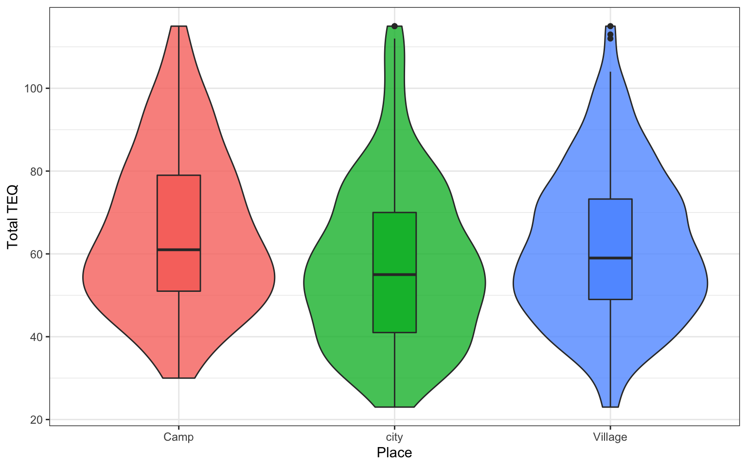

Figure 4.2: TEQ Scores

From looking at the graph we just created, what location tends to have highest TEQ?

Village Camp City

4.7 Recoding Factors

The original file has Camp, city, Village. It might be neater to have Camp, City, Village. We can easily recode the city level of the Place factor using the following code.

If you re-run the code for the graph now, this should be updated.

total_TEQ <- total_TEQ %>%
    mutate(Place = recode(Place, city = "City"))

4.8 Simple Network

When creating a network, it is important to think about how complex it will be. The higher the number of nodes being examined, then the higher the number of edges have to be estimated. Too many nodes results in networks that are unstable.

In this example, we will create a simple network from the single question items of the PAQ (Parental Authority Questionnaire).

First, we will select the PAQ items from data_factors:

PAQ <- data_factors %>%
  select(PAQ1:PAQ11)

Like all statistical techniques that use sample data to estimate parameters, the correlation and partial correlations values will be influenced by sampling variations and exact zeros will be rarely observed in the matrices. Consequently, correlation networks will nearly always be fully connected networks, possibly with small weights on many of the edges that reflect weak and potentially spurious partial correlations.

Spurious relationships will be problematic in terms of the network interpretation and will compromise the potential for network replication. In order to limit the number of such spurious relationships, a statistical regularisation technique, which takes into account the model complexity, is frequently used.

The LASSO regularisation yields a more parsimonious network (fewer connections between nodes), assumed to reflect only the most “important” empirical relationships in the data. The LASSO utilizes a tuning parameter λ (lambda) that controls the level of sparsity. The tuning parameter directly controls how much the likelihood is penalized for the sum of absolute parameter values. When the tuning parameter is low, only a few edges are removed, likely resulting in the retention of spurious edges. When the tuning parameter is high, many edges are removed, likely resulting in the removal of true edges in addition to the removal of spurious edges. EBICglasso sets a tuning parameter of 0.5 by default.

Network <- estimateNetwork(PAQ, default = "EBICglasso", corMethod = "cor_auto")

The size and density of the edges between the nodes respresent the strength of connectedness. Positively related nodes are shown in blue and negatively related nodes are shown in red.

plot(Network, layout="spring", labels=colnames(PAQ))

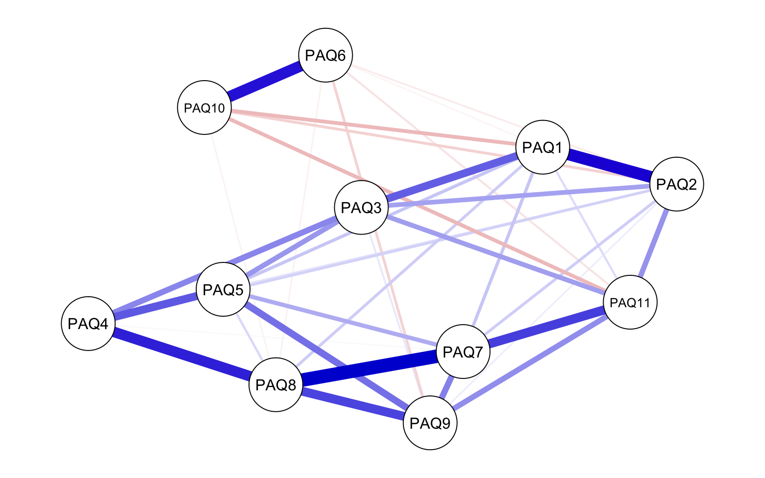
Figure 4.3: PAQ Network Graph

4.9 Interpretation

Parental Authority Questionnaire (PAQ)

1. My family Knows what I do in my free time
2. My family knows friends I have during my free time
3. My family knows how I spend my money
4. My family knows the time of my exams
5. My family knows what I do at school
6. During the past month, my family has no idea if I was at home in the evenings
7. Usually I tell my family about school
8. Usually I tell my family about exams
9. Usually I tell my family about my relationships with teachers
10. Usually I conceal from family a lot of things which I do in the evening
11. When I am out, I tell my family what I did after coming home

The network shows the strength of relationships between the variables. Some variables have quite strong connections (e.g. PAQ8 and PAQ7), whereas others have weak relationship (e.g. PAQ8 and PAQ10). Visual inspection of the network suggests that some variables may be related. However, visual inspection of the graphical display of complex relationships requires careful interpretation, especially if there are a large number of nodes in the network. Borsboom (Borsboom, 2016) recommends exploratory network analysists start by creating manageable networks because too many nodes can lead to a dense network which is difficult to make sense from.

A key concept in network analysis is the centrality of the symptom: if a behaviour or symptom (e.g. fatigue) has many and/or strong associations to other nodes, they are more central within the network than a less connected symptom.There are different centrality metrics, and strength most often used. Expected influence is related to strength but argued to sometimes be a better metric

From looking at strength, it appears PAQ7 and PAQ8 have the strongest influence on the nodes in the network. How might we interpret this? Network analysis is purely statistical, the measurement and inclusion of nodes depend on your theory / research question.

centralityPlot(Network, include = c("Strength"),
               orderBy = "Strength")

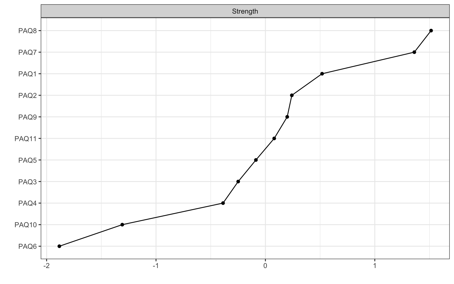
Figure 4.4: Centrality Plot

4.10 Assumptions

Network Analysis assumes normally disturbuted data which can be rare in psychology where Likert scales (such as that used to measure data here) are common.

“our data did not meet all assumptions of multivariate normality. This is not unusual in psychology, but as it is unclear at present how robust the employed methods are to such violations, results need to be interpreted with caution.” (Aalbers, 2019)

4.11 Stability

When are estimating networks, we are estimating a structure. While we end up with a model, there is uncertainty about model parameters. Researchers in Amsterdam have developed a bootstrapping procedure so we can estimate stability with more confidence. For more information on this, please see a tutorial by Eiko Fried.